
Amplitude Modulation (AM) is one of the foundational techniques in analog communication systems and electrical engineering education. While commercial broadcasting has increasingly migrated toward frequency modulation and digital protocols, AM remains the primary pedagogical bridge connecting time-domain signal multiplication with frequency-domain spectral translation.
Textbooks often introduce amplitude modulation through static graphs of sinusoidal envelopes and trigonometric formulas. However, genuine intuitive understanding comes from actively manipulating signal parameters: sweeping the modulation depth, witnessing an envelope cross zero into overmodulation distortion, inspecting the carrier and sideband power spikes on an FFT spectrum analyzer, and listening to or observing the recovered message after envelope detection.
In this tutorial, we examine the mechanics of amplitude modulation, calculate the modulation index and sidebands, analyze why overmodulation corrupts envelope detection, and demonstrate how to simulate and demodulate AM signals online using CircuPilot Signal Lab.
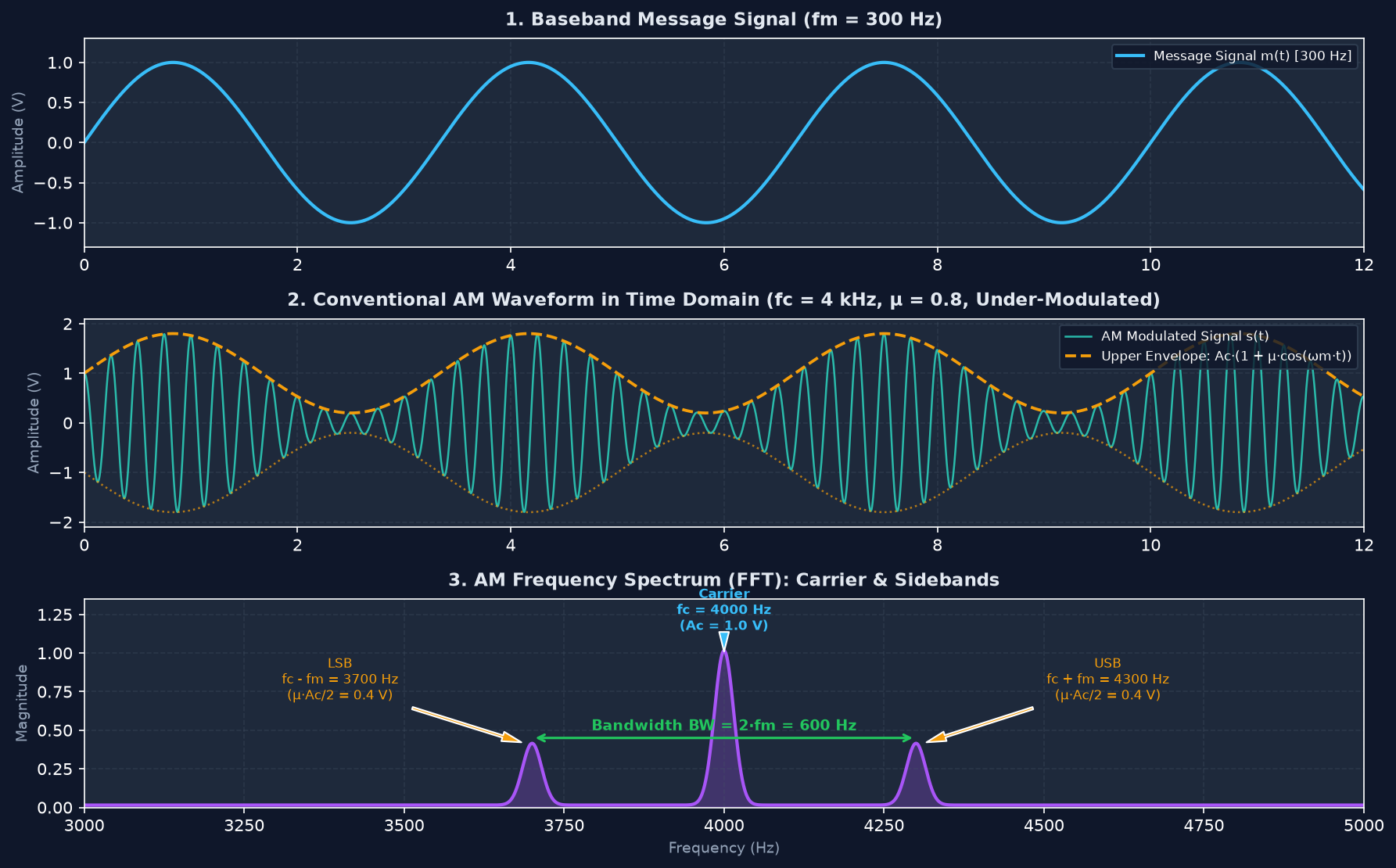
1. What Is Amplitude Modulation (AM)?
In analog communications, baseband information—such as voice, music, or telemetry data—cannot be broadcast directly over long distances because radiating low frequencies requires impractically large antennas. An efficient antenna typically requires a physical length proportional to a quarter of the radiated wavelength (λ = c / f). Transmitting a 300 Hz audio tone directly would necessitate an antenna over 250 kilometers long.
Amplitude Modulation circumvents this physical limitation by using the low-frequency message to vary the instantaneous amplitude of a high-frequency radio frequency (RF) carrier signal:
- Message Signal (m(t)): The information signal to transmit, characterized by baseband frequency fm and peak amplitude Am.
- Carrier Signal (c(t)): A high-frequency sinusoidal oscillation with carrier frequency fc and amplitude Ac, where fc >> fm.
- Modulated Waveform (s(t)): The composite transmitted signal whose outer amplitude boundary—called the envelope—mirrors the original baseband information.
2. The Mathematical Model of an AM Signal
For a sinusoidal message and carrier, a conventional Double-Sideband Large-Carrier (DSB-LC) amplitude modulated wave is defined as:
s(t) = Ac · [1 + μ · cos(2π · fm · t)] · cos(2π · fc · t)Where:
- Ac is the peak amplitude of the unmodulated carrier.
- fc is the carrier frequency in Hertz.
- fm is the message frequency in Hertz.
- μ is the dimensionless modulation index (also represented by m or ka·Am).
Because the carrier frequency fc is typically orders of magnitude higher than the message frequency fm, the carrier acts as a high-frequency vehicle transporting the slow-varying envelope through the transmission medium.
3. Understanding the AM Modulation Index (μ)
The modulation index μ measures the depth or intensity of amplitude modulation. For a single sinusoidal modulating tone, it represents the ratio of peak message amplitude to carrier amplitude:
μ = Am / AcWhen analyzing an AM waveform on an oscilloscope, measuring Am and Ac directly can be challenging once the carrier is modulated. Instead, μ is determined from the maximum envelope peak (Vmax) and minimum envelope trough (Vmin):
Vmax = Ac · (1 + μ)
Vmin = Ac · (1 - μ)
μ = (Vmax - Vmin) / (Vmax + Vmin)
Three Critical Modulation Conditions
The numerical value of μ establishes three distinct operating regimes:
- Under-Modulation (μ < 1, e.g., μ = 0.5 to 0.8): The carrier amplitude varies in proportion to the message, but the envelope never touches or crosses the zero axis (Vmin > 0). The envelope cleanly tracks the shape of m(t), allowing a simple diode envelope detector to recover the audio signal with zero distortion.
- 100% Modulation (μ = 1.0): The modulation depth reaches its theoretical upper limit for envelope detection. At the trough of the message cycle, Vmin touches exactly 0 V. Signal-to-noise ratio and sideband power efficiency are maximized without clipping.
- Overmodulation (μ > 1, e.g., μ = 1.4): When the modulating amplitude exceeds the carrier amplitude, the term [1 + μ · cos(2π · fm · t)] becomes negative during part of the audio cycle. This causes the high-frequency carrier to undergo an abrupt 180° phase inversion. Because standard diode envelope detectors respond only to the absolute magnitude |s(t)|, the negative lobes invert upward. This chops the bottom of the recovered waveform, introducing severe harmonic distortion.
4. What Are AM Sidebands?
A common misconception among beginners is that amplitude modulation merely changes a carrier's amplitude without altering its frequency content. In reality, multiplying two time-domain sinusoids generates new frequencies in the frequency domain.
Applying the trigonometric identity cos(A) · cos(B) = 0.5 · [cos(A + B) + cos(A - B)] expands the standard AM equation into three distinct spectral tones:
s(t) = Ac·cos(2π·fc·t) + (μ·Ac/2)·cos(2π·(fc - fm)·t) + (μ·Ac/2)·cos(2π·(fc + fm)·t)The resulting spectrum contains three components:
1. Carrier: Located at fc with amplitude Ac. It conveys no message information on its own, but provides the reference vector required for simple asynchronous rectification.
2. Lower Sideband (LSB): Located at fc - fm with amplitude (μ · Ac) / 2.
3. Upper Sideband (USB): Located at fc + fm with amplitude (μ · Ac) / 2.
Both sidebands carry the exact same informational content of the original message, mirrored symmetrically on either side of the carrier.
Numerical Example and Transmission Bandwidth
Consider a standard AM broadcast scenario where:
- Carrier frequency:
fc = 100 kHz - Message frequency:
fm = 5 kHz - Modulation index:
μ = 0.6
| Component | Frequency | Amplitude Formula | Numerical Amplitude |
|---|---|---|---|
| Lower Sideband (LSB) | 95 kHz (fc - fm) | (μ · Ac) / 2 | 0.30 · Ac |
| Carrier | 100 kHz (fc) | Ac | 1.00 · Ac |
| Upper Sideband (USB) | 105 kHz (fc + fm) | (μ · Ac) / 2 | 0.30 · Ac |
The required transmission bandwidth is:
BW = 2 · fmIn this example, the required transmission bandwidth is BW = 2 · 5 kHz = 10 kHz. For a complex message containing multiple frequencies (such as speech from 300 Hz to 3400 Hz), the total RF bandwidth is always twice the highest frequency component: BW = 2 · fm,max.
5. AM Demodulation: Recovering the Original Message
Modulation is only the first half of a communication link. At the receiver, the original baseband information must be extracted from the high-frequency RF carrier. This process is called demodulation or detection.
The Diode Envelope Detector (Asynchronous)
The simplest and most widely used demodulator is the diode envelope detector:
- A semiconductor diode rectifies the incoming AC signal, blocking negative half-cycles.
- An RC parallel low-pass filter smooths the remaining positive RF pulses. The capacitor charges quickly to the peak carrier voltage and discharges slowly through the resistor, following the envelope contour while filtering out the high-frequency carrier ripple.
When the modulation index is within the normal operating range (μ ≤ 1.0), the envelope voltage faithfully tracks the original message.
Why Overmodulation Causes Distortion
When μ > 1, the mathematical envelope dips below zero. Because an envelope detector acts as an absolute value rectifier (|s(t)|), it cannot detect the 180° carrier phase inversion. The portion of the message below zero is mirrored into positive voltage territory, creating a sharp cusp where a smooth trough should be.
To recover overmodulated transmissions or Double-Sideband Suppressed-Carrier (DSB-SC) signals, receivers must use coherent synchronous demodulation. This technique multiplies the received signal by a locally generated carrier synchronized in frequency and phase (s(t) · cos(2π·fc·t)), followed by a low-pass filter.
6. Hands-On Experiment: Simulate AM in CircuPilot Signal Lab
Try it live: Open CircuPilot Signal Lab and click the "2. AM Comm" template button to run this complete AM modulation and demodulation experiment interactively in your browser.
Observing AM waveforms and spectra dynamically makes the mathematical relationships immediately apparent. You can experiment with these parameters without physical hardware using CircuPilot Signal Lab.
CircuPilot Signal Lab is a browser-based visual laboratory built on NumPy and SciPy. It provides dedicated DSP blocks, real-time dual-trace oscilloscopes, and 2048-point FFT spectrum analyzers.
Step-by-Step AM Transceiver Walkthrough
1. Open CircuPilot Signal Lab in your browser.
2. In the template bar at the top of the canvas, click "2. AM Comm".
3. The platform automatically instantiates and wires a complete communications chain:
- Message Generator (
analogGen): 300 Hz sinusoidal baseband tone, amplitude 1.0 V. - AM Modulator (
amMod): Carrier frequencyfc = 4000 Hz, modulation indexμ = 0.8, modedsb-lc. - AM Demodulator (
amDemod): Envelope detector with an 800 Hz 4th-order Butterworth low-pass filter. - Dual-Trace Oscilloscope (
oscilloscope): CH1 connects to the modulated AM output; CH2 connects to the demodulated audio output. - FFT Spectrum Analyzer (
spectrum): Displays real-time linear and decibel magnitude spectra.
Key Observations to Verify:
- Carrier and Sideband Spacing: Look at the FFT spectrum analyzer. You will see three distinct spikes: the primary carrier at 4000 Hz, the lower sideband at 3700 Hz, and the upper sideband at 4300 Hz. The distance between the sidebands is exactly
2 · fm = 600 Hz. - Testing Overmodulation: Select the AM Modulator block on the canvas to open the sidebar inspector. Change
modulation_indexfrom0.8to1.4. On CH1 of the oscilloscope, observe how the envelope pinches to zero and inverts. Look at CH2: the recovered 300 Hz sine wave exhibits clipped, flattened troughs, and harmonic distortion peaks emerge across the FFT spectrum. - Double-Sideband Suppressed-Carrier (DSB-SC): In the AM Modulator inspector, switch
am_typefromdsb-lctodsb-sc. In the FFT spectrum, the 4000 Hz carrier peak disappears completely, leaving only the two information sidebands. Notice how the envelope detector on CH2 output drops to zero/hash, demonstrating why DSB-SC requires coherent synchronous demodulation rather than simple envelope detection.
7. Common Questions About AM Modulation
What is the modulation index in AM?
The modulation index (μ) measures the depth of amplitude variation relative to the unmodulated carrier amplitude. For a sinusoidal message, it is calculated as μ = Am / Ac. When observing oscilloscope peaks and troughs, it is calculated as μ = (Vmax - Vmin) / (Vmax + Vmin).
What happens when the modulation index is greater than 1?
When μ > 1, the condition is known as overmodulation. The envelope crosses zero and inverts its phase during part of the modulating cycle. A conventional envelope detector rectifies this negative swing, creating severe acoustic harmonic distortion and adjacent-channel spectral splatter.
What are the upper and lower sidebands?
Sidebands are new frequency components generated by multiplying the baseband message with the RF carrier. For a single-tone message, the Lower Sideband occurs at fc - fm and the Upper Sideband occurs at fc + fm. Both sidebands carry identical message information.
What is the bandwidth of a conventional AM signal?
For a baseband message with maximum frequency fm,max, the transmission bandwidth required by a double-sideband AM signal is BW = 2 · fm,max.
What is the difference between AM modulation and demodulation?
Modulation combines a low-frequency baseband message with a high-frequency RF carrier at the transmitter for antenna radiation. Demodulation extracts the original baseband audio or data signal from the modulated carrier at the receiver.
Can AM modulation be simulated online?
Yes. Interactive browser-based environments like CircuPilot Signal Lab allow you to construct AM transmitters, vary modulation index, inspect real-time FFT spectra, and compare envelope versus coherent detection without physical hardware or software installation.
Conclusion
Amplitude modulation demonstrates how time-domain signal multiplication translates information into sidebands across the frequency spectrum. Maintaining the modulation index between 0 and 1 ensures clean, distortion-free envelope detection while maximizing transmission signal-to-noise ratio.
By experimenting with real-time waveform parameters in CircuPilot Signal Lab, you can visualize sideband spacing, examine overmodulation clipping, and test demodulator performance firsthand. For component-level implementations—such as diode envelope detector circuits, LC tank tuners, and passive low-pass filters—you can model the underlying circuit schematics in the CircuPilot Circuit Simulator.
Frequently asked questions
What is the modulation index in AM?
The modulation index (μ) is the ratio of peak message amplitude to carrier amplitude (μ = Am / Ac). It measures modulation depth, where μ < 1 is under-modulation, μ = 1 is 100% modulation, and μ > 1 causes overmodulation and envelope clipping.
What happens when the modulation index is greater than 1?
When the modulation index exceeds 1 (μ > 1), the envelope term 1 + μ·cos(ωm·t) crosses zero and becomes negative. A standard envelope detector rectifies this negative swing, creating severe harmonic distortion in the recovered audio signal.
What are the upper and lower sidebands?
They are the frequency components located above and below the carrier frequency. For a single-tone message, they occur at fc + fm (Upper Sideband) and fc - fm (Lower Sideband).
What is the bandwidth of a conventional AM signal?
For a message with maximum frequency fm,max, the required transmission bandwidth is BW = 2 · fm,max.
What is the difference between AM modulation and demodulation?
Modulation combines a low-frequency information message with a high-frequency carrier for transmission. Demodulation extracts the original baseband message from the received modulated signal.
Can AM modulation be simulated online?
Yes. CircuPilot Signal Lab provides an interactive, zero-install browser environment to generate, modulate, filter, demodulate, and analyze AM signals in both time and frequency domains.